Snap to Fit

In the plot below, the teal scan is the target. It stays fixed. The orange scan is the source: the same room, moved by a rigid motion that we do not know. A rigid motion moves every point the same way:

Here \(R\) is a rotation matrix and \(t\) a translation vector. Distances and angles do not change, so the scan moves as one solid piece. In 2D the motion has 3 degrees of freedom: one angle and two shifts. In 3D it has 6: three for rotation and three for translation.

For now, assume we also know which source point goes with which target point: \(a_i \leftrightarrow b_i\) for \(i = 1, \dots, n\). The best motion brings matched points as close as possible on average:

The constraints say that \(R\) is a rotation. \(R^\top R = I\) keeps lengths and angles. \(\det R = +1\) rules out mirror images, which also keep lengths but cannot come from moving a real sensor. The square root of the cost is the root-mean-square error (RMSE) between matched points, in metres.

Why rotation is the hard part

Fix \(R\) and the cost is a quadratic in \(t\). That is ordinary least squares, with a one-line answer. The rotation is different. Its entries must satisfy \(R^\top R = I\), which is a set of quadratic equations, so the allowed matrices form a curved set. A simple test shows the problem: the average of two rotations is not a rotation.

This matrix turns vectors by 45° and also shrinks them by 29%. If we solved for the four entries of \(R\) by plain least squares, we would get a matrix like this one that can stretch, shrink or shear the scan. The constraint makes the problem nonlinear.

Even so, there is an exact answer in closed form, with no initial guess and no iterations. Step 02 builds it from two averages and one SVD.

Why the recipe works, in brief

Translation only moves the centroid, so centring removes it from the problem. The best rotation then depends on the pairs only through \(M\), and the SVD of \(M\) splits it into directions in the source (\(V\)), directions in the target (\(U\)) and how strongly each pair agrees (\(\Sigma\)). Turning \(V\) onto \(U\) is the answer, with one sign check so that \(R\) stays a rotation. Step 03 proves each claim.

How many matches are needed? Two distinct points fix a 2D motion, and three points that are not on one line fix a 3D motion. More matches average out the noise. The final RMSE is the error that no rigid motion can remove.

Arun, Huang and Blostein (1987) published this SVD recipe for 3D point sets. The determinant fix comes from Kabsch (1976, 1978) and Umeyama (1991). The course states the problem on W4 · slides 24–25 and asks you to know how to derive it W5 · “Next week”.

The sign game

Line 7 says the best \(S\) is \(I\). Line 9 says a rotation sometimes has to flip one sign. Both winners are diagonal sign matrices, so the eight patterns \(S = \operatorname{diag}(\pm 1, \pm 1, \pm 1)\) below are enough to see the whole story. Here \(M\) is a fixed \(3 \times 3\) example, factored in your browser with the same SVD code as Step 02. Pick the signs \(s_1, s_2, s_3\) and watch the score and the determinant.

The table makes the rule concrete. Every flip costs \(2\sigma_i\) of score, and every flip changes the sign of \(\det R\). When \(\det(UV^\top) = -1\), an odd number of flips is needed, and the cheapest is the single flip on the smallest \(\sigma\). When \(\det(UV^\top) = +1\), no flip is needed and \(S = I\) wins outright.

One more view of the same answer: \(M = U\Sigma V^\top = (UV^\top)(V\Sigma V^\top)\) is the polar decomposition of \(M\), an orthogonal factor times a symmetric positive semidefinite one. The slide's \(R = UV^\top\) is that orthogonal factor.

In symbols, ICP looks for the rotation \(R\) and translation \(t\) that minimise the mean squared distance from each moved orange point to its nearest teal point:

The \(a_i\) are the \(N\) orange points (source scan \(A\), which moves) and the \(b_j\) are the teal points (target scan \(B\), which stays put). If you knew which \(j\) wins each min, this would be exactly the problem from Step 02. ICP takes turns: fix the pose and choose the pairs, then fix the pairs and choose the pose.

1. Match. For every \(i\), find \(c(i) = \arg\min_j \lVert R\,a_i + t - b_j \rVert\). A k-d tree over the teal points answers each query in roughly logarithmic time instead of checking every teal point.
2. Reject (optional). Keep \(K = \{\, i : \lVert R\,a_i + t - b_{c(i)} \rVert \le d_{\max} \,\}\). A very long pair is usually a wrong pair or an outlier. With no cutoff, \(K\) holds every \(i\).
3. Solve. \((R, t) \leftarrow \arg\min_{R,\,t} \sum_{i \in K} \lVert R\,a_i + t - b_{c(i)} \rVert^2\). This is Procrustes with known pairs. Let \(\mu_A\) be the mean of the kept \(a_i\) and \(\mu_B\) the mean of their matches. Take the SVD \(M = \sum_{i \in K} (b_{c(i)} - \mu_B)(a_i - \mu_A)^\top = U \Sigma V^\top\), then \(R = U D V^\top\) with \(D = \operatorname{diag}(1, \det(UV^\top))\), and \(t = \mu_B - R\,\mu_A\).
4. Move and repeat. Apply the new \(R, t\) to the orange scan and go back to 1. Stop when \(E\) stops dropping.

The page made both scans from the same shape, then rotated and shifted the orange one, so it knows the true transform. The two error readouts compare ICP's estimate with that truth. RMSE is the square root of \(E\), taken over the kept pairs only. Overlap crops the two scans from opposite sides, the way a robot that has driven on sees only part of its old view. Points that only one scan sees have no true partner, so they act like outliers. At 80% overlap, plain ICP already stops almost half a metre from the truth.

TryRaise the initial rotation a few degrees at a time and press Play after each change. The room still finds its way home from 75°, though it needs about 70 iterations. At 76° it locks onto a pose about 68° off and stays there. Now go the other way: it already fails at −38°.

TrySet outliers to 30% and press Play. The random orange points drag the result almost 4° off. Now move the cutoff to 0.20 m and press Play again. ICP carries on from where it stopped, drops the long pairs, and lands on the true pose.

TryPick the star, set the rotation to 40° and press Play. ICP ends with an RMSE of 0.026 m, as low as a correct fit (run 30° to compare), yet the rotation error is 72°. The star looks the same every 72°, so \(E\) can barely tell those poses apart.

Why the error never goes up

Track the sum of squared pair lengths, \(\sum_i \lVert R\,a_i + t - b_{c(i)} \rVert^2\). Each iteration changes it twice, and neither change can raise it.

• Matching gives every orange point its nearest teal point. No pair can be longer than the one it replaces.
• Solving finds the exact minimum of this sum for the current pairs. The old pose was one of the candidates, so the new sum is no larger.

Right after matching, the sum is exactly \(N\,E(R, t)\), so \(E\) never goes up either. It is never negative, and a sequence that never increases and is bounded below must settle. Besl and McKay (1992) proved this monotone convergence for ICP. You can see it in the chart: with the cutoff off, the curve never rises.

\(E\) also never reaches zero, even at the true pose. The two scans sample the walls at different spots, so each orange point sits a few centimetres from the nearest teal sample. Step 06 measures the distance to the wall's line instead, which removes most of this floor.

It converges, but only to a local minimum

The theorem says the error stops dropping. It says nothing about where. ICP only ever looks at nearest neighbours, so it slides downhill from the starting pose and settles in the valley of \(E\) it started in: a local minimum. If it starts too far off, walls pair with the wrong walls and ICP settles on a wrong pose. This page can tell, because it knows the truth. A robot only sees the RMSE, and a wrong fit can have a low RMSE, as the star shows. Step 05 maps out which starting poses work.

Outliers and partial overlap cause a second kind of failure. They move the minimum of \(E\) itself, so ICP drifts away even from a perfect start. Set the rotation and offset to 0 and the outliers to 30%: ICP still ends about 3° off. A better first guess cannot fix that. Dropping the long pairs can, as the second Try above shows. The status line under the buttons says which kind of failure you are looking at.

Where the first guess comes from

Real systems rarely start ICP blind. The first guess comes from something cheaper:

• Odometry or an IMU. Wheel encoders and a gyro already say roughly how far the robot moved and turned since the last scan.
• The previous frame. A depth camera at 30 Hz barely moves between frames, so the last pose, or a constant-velocity prediction from it, is already close. KinectFusion (Newcombe et al. 2011) starts each frame's ICP from the previous frame's pose.
• Feature matches with RANSAC. Match distinctive keypoints between the scans and fit a rough \(R, t\) that survives the wrong matches. W5 · RANSAC

ICP then does the part it is good at: turning a rough guess into a precise one.

Teal is the fixed scan, orange the scan that moves, grey lines the current nearest-neighbour pairs. Hollow orange points in B are points the cutoff left unpaired. Arrows in C mark the moving scan's frame: solid where ICP put it, dashed where it truly is.

The basin of convergence

Card A was one bad start. To see the whole picture, run ICP from many starts and colour each one by where it ended. Each cell below is one complete run on 150 points: ICP iterates until the error stops dropping, at most 100 times. The moving scan starts turned by the column's angle and shifted by the row's distance, always in the same direction (35° above the x-axis). Green means ICP reached the true pose: rotation error under 2° and translation error under 5 cm. Red means it stopped somewhere else; the stronger the red, the larger the final error.

TryPick the star. Every red cell is now hatched. Hover a few: each of those runs ended 72° or 144° from the truth, a fifth or two fifths of a turn. The star looks the same after that turn, so the wrong pose fits just as well as the right one.

With every pair kept, the start rotation matters far more than the start offset. Each Procrustes step puts the centroid of the moving scan onto the centroid of its matched points, and those points all lie on the target. So even from 2.5 m away, the first iteration removes a quarter to a half of the shift, and the next ones keep closing the gap. A large turn is harder. The nearest-neighbour guesses are then wrong in a consistent way, and Procrustes solves exactly the problem it is given.

Now set the pair cutoff to 0.5 m. Far starts leave few pairs inside the cutoff, so the basin shrinks. The room now reaches the truth from 38 of 264 starts instead of 87. The star reaches it from 20 instead of 54, and only from offsets of 1 m or less. The kind of cutoff that rescued card B costs reach here.

TryPress Play and watch the left scan inch along the walls while the right one snaps into place. Then tick Show normals: the right panel measures every residual along those short ticks, and nothing along the wall.

Why point-to-plane becomes a linear problem

Point-to-point has the closed-form Procrustes answer from Step 02. Point-to-plane has none. The proof in Step 03 used the fact that a rotation keeps lengths, \(\lVert R a_i \rVert = \lVert a_i \rVert\). The squared term then did not depend on \(R\), and one SVD maximised what was left. The part of \(R a_i\) along a fixed normal, \((R a_i)^\top n_i\), does change with \(R\), so its square stays in the cost and that step fails. Low (2004) linearises the problem instead W5 · slides 54–55.

Within one iteration, let \(a_i\) be where each moving point sits now, so \(R\) and \(t\) are only this iteration's correction. That correction is small, so the rotation is close to the identity: \(R \approx I + [\boldsymbol\omega]_\times\), where \([\boldsymbol\omega]_\times\) is the cross-product matrix of a small rotation vector \(\boldsymbol\omega\). Substitute it and use \((\boldsymbol\omega \times a_i)^\top n_i = \boldsymbol\omega^\top (a_i \times n_i)\). Each residual becomes linear in the unknowns:

That is ordinary linear least squares. Solve the normal equations \(\big(\sum_i J_i J_i^\top\big)\, x = -\sum_i J_i\, r_i\), turn \(\boldsymbol\omega\) back into an exact rotation, apply it, match again, and repeat. In 3D, \(x\) has 6 unknowns: 3 for \(\boldsymbol\omega\) and 3 for \(t\). In 2D the rotation is a single angle \(\theta\), \(a_i \times n_i\) becomes the scalar \(a_{i,x} n_{i,y} - a_{i,y} n_{i,x}\), and there are 3 unknowns.

Where the normals come from

Take the \(k\) nearest target points around \(b_i\) (here \(k = 6\)), subtract their centroid, and run PCA. The direction of smallest spread is the normal. This is the total least squares fit that the lecture calls orthogonal regression W5 · slides 27–30: the best line or plane through a cloud passes through its centroid, and its normal is the eigenvector of the scatter matrix with the smallest eigenvalue, the PCA-based solution. The residual \(\epsilon_i = n^\top (p_i - q)\) on those slides is the same quantity point-to-plane ICP minimises.

The catch

• It needs normals. That is one small PCA per target point. For a fixed target you compute them once.
• Bad normals mislead it. On noisy or curved patches the PCA normal tilts, and the error is then measured in a slightly wrong direction. Point-to-point uses no normals, so it has no such failure.
• The step is a linearisation. It is accurate only for small rotations. ICP relinearises at every iteration, so near the answer this costs nothing, but a far start makes each step less reliable.
• Flat scenes leave it blind. In the corridor of Step 05, every normal points across the hall, so the entry of \(J_i\) that multiplies the shift along the corridor is zero for every pair. The matrix \(\sum_i J_i J_i^\top\) is then singular in that direction (nearly singular once noise tilts the normals): the same blind spot, now visible in the algebra.

The same race on real 3D data

Stanford Bunny, scan bun045 onto bun000 (true rotation 34.3°; 1,811 and 1,919 points after a 4.2 mm voxel grid). Both methods start from the identity with a 1 cm correspondence cutoff. Errors are measured from the scanner's ground truth, and Open3D ran the same setup as a cross-check.

Point-to-plane stopped on its own after 19 iterations. Point-to-point used all 60 we allowed and still ended more than 20 times further off in rotation. A scanned surface is mostly smooth patches, which is exactly where sliding along the surface pays off.

How the error is measured

ICP returns a pose \((\hat R, \hat t)\) that maps source points into the target frame. We compare it with the ground-truth pose \((R_{gt}, t_{gt})\):

\(e_R\) is the angle of the leftover rotation \(R_{gt}^\top \hat R\). The RMSE in the readout is something else: the root-mean-square distance between matched points, over the pairs inside the cutoff. It needs no ground truth, which is why ICP can report it, and also why it can mislead.

The bunny: two views of one ceramic rabbit

The Stanford Bunny is a small ceramic rabbit, scanned with a laser range scanner at Stanford in 1994. A range scanner only sees the side facing it, so the bunny was turned between scans. We use two of its ten scans: bun000 as the target and bun045 as the source. The names suggest 0° and 45°. The alignment file that ships with the scans, bun.conf, puts the true rotation between them at 34.3°, and that file is our ground truth.

The two scans cover different parts of the surface. A point on a patch that only one scan sees has no true partner in the other, so its closest-point match is wrong by construction. That is why ICP here ignores any pair more than 1 cm apart (the correspondence cutoff). Both scans were thinned with a 4.2 mm voxel grid, which replaces the points inside each 4.2 mm cube by their average: 1811 source points and 1919 target points remain.

Point-to-plane lands 0.10° from the ground truth in 19 iterations. Point-to-point is still 2.18° off when it reaches the 60-iteration cap, which Open3D used too. The two scans sample the surface at different spots, so no source point has an exact twin in the target. Point-to-point pulls each point toward a neighbour that is not its twin, and the best fit to those pairs sits about 2° from the truth. Start it at the ground-truth pose and it walks away again, to 1.90° off. The run from the identity is heading for that same pose: without the cap it gets there after 77 iterations. Point-to-plane only counts distance along the surface normal, so a point can slide along the surface for free. That is the right model for two samplings of one surface (Step 06).

Now look at the RMSE readout. Point-to-point ends at 2.32 mm and point-to-plane at 2.23 mm. One pose is 2.18° off and the other 0.10°, yet the residuals differ by less than 0.1 mm. A 2° error barely moves the residual, so a low RMSE does not prove that a pose is right. Only an independent ground truth can show that.

The desk: two Kinect frames, 0.2 s apart

The TUM RGB-D benchmark (Sturm et al., 2012) filmed indoor scenes with a handheld Microsoft Kinect while a motion-capture system tracked markers on the camera. We take two frames of the fr1/desk sequence. Between them the camera turned 9.19° and moved 8.61 cm. The light-blue book on the left of the desk is Multiple View Geometry by Hartley and Zisserman.

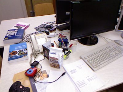
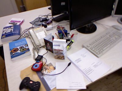
Colour frames from TUM RGB-D fr1/desk (Sturm et al., IROS 2012), CC BY 4.0, shown at reduced size. Timestamps are the dataset's colour-image times.

From depth pixels to 3D points

A Kinect returns a colour image and a depth image. Each depth pixel \((u, v)\) holds a 16-bit value \(d\), and in this dataset 5000 units are one metre. The pinhole model W1 camera model projects a 3D point to \(u = f_x X/Z + c_x\) and \(v = f_y Y/Z + c_y\). The depth image tells us \(Z\), so we can run the model backwards W6 RGB-D:

with the published calibration of this camera: \(f_x = 517.3\), \(f_y = 516.5\), \(c_x = 318.6\), \(c_y = 255.3\), all in pixels. One 640 × 480 frame gives up to 307,200 points. We keep every second pixel in each direction, drop depths outside 0.3 to 3.5 m, and thin the rest with a 2.5 cm voxel grid. That leaves 4718 target points and 4291 source points, each with a colour from the RGB image. The points live in the camera frame (\(x\) right, \(y\) down, \(z\) forward). The viewer turns them so that up is up, and draws each camera as a small pyramid.

Why ICP stops 1.5° from motion capture

Both ICP variants end 1.4° to 1.5° and 1.6 to 1.8 cm from the motion-capture pose. Is ICP stuck in a bad local minimum? Start it at the motion-capture pose itself and it walks away to the same answer: 1.45° and 1.56 cm here, 1.45° and 1.58 cm in Open3D. You can check this above: pick Start from: Ground truth and run point-to-point. The RMSE falls from 1.61 cm at the mocap pose to 1.44 cm. With a 6 cm cutoff the scans fit best about 1.5° from the mocap pose, and ICP finds that pose from either start. So the gap is not a local minimum. It has two other sources.

The cutoff. The camera moved, so each frame sees some of the desk that the other does not. Points there have no true partner. Each cloud fills its own camera's view, so their closest-point pairs pull the estimate back toward no motion, and a looser cutoff lets more of them count. With a 2 cm cutoff, point-to-plane ends 1.07° and 1.34 cm from mocap, from either start. With 20 cm it ends 2.23° off. Try cutoffs between 2 and 20 cm with point-to-plane and watch the camera-motion rows in the readout.

The ground truth. About 1° remains even at 2 cm. There ICP measures a turn of 8.18° and a move of 7.79 cm, where mocap says 9.19° and 8.61 cm. The two agree on the axis of the turn to within 3°, but not on its size. That rules out one suspect. Mocap tracks markers on the Kinect's body, and a calibrated transform \(X\) takes the marker pose to the camera. If the markers move by \(A\), the camera moves by \(B = X^{-1} A X\), the hand-eye relation \(AX = XB\) W4 slides 22–25. A change of frame keeps the rotation angle, so an error in \(X\) could tilt the axis of the turn but not change its size.

Timing can change the size. If the camera moved at a steady 46°/s and 43 cm/s, the missing 1.0° and 0.8 cm are both about 20 ms of motion. Timestamps are not that exact: mocap runs at 100 Hz and we take the sample nearest each depth image, and the Kinect's own two streams are not synchronised (each depth image here was stamped 13 to 15 ms after its colour image). Our back-projection also ignores the lens distortion that TUM publishes for this camera, which bends both clouds slightly. Two frames cannot separate these causes.

And the code? On this pair, this page's point-to-point ICP and Open3D's end within 0.02° and 0.05 cm of each other. Both implementations find the same minimum of the same cost. The gap to mocap comes from a choice inside that cost, the cutoff, and from the limits of the ground truth.

TryPlay the first three rounds. In round 2 ICP gets stuck far from the answer. In round 3 ICP, and most likely you too, lands on a pose that scores as well as the true one and is still wrong. After each round, pick ICP from yours to run ICP from your rough fit.

What the game shows

ICP is a local method. Neither of its two steps can raise the nearest-neighbour error, so it slides downhill from wherever it starts (Besl & McKay 1992). From a close start it ends far more precisely than a hand fit, because every iteration solves the Procrustes problem for all matched pairs at once.

From a far start, many first matches are wrong. ICP then settles in the valley of the error it started in, which need not be the deepest one. You see the whole shape at once, so you rarely fall into that trap. Real systems split the work the same way: a rough initial guess from odometry, an IMU or a global feature match, then ICP to refine it.

Check yourself

Eight questions on the whole page. Pick an answer to see why it is right or wrong.

Slide map

Where each step of this page sits in the course.

How we verified

We ran the same tests in Python (numpy and Open3D 0.20, on the team's Jetson AGX Thor) and with this page's JavaScript. Errors are against ground truth: the scanner's alignment for the Bunny, motion capture for TUM.

• Bunny. Stanford scans bun045 (moves) and bun000 (fixed), 4.2 mm voxel grid, 1811 and 1919 points, true rotation 34.3°. Ground truth comes from the scanner's bun.conf, which stores the conjugate rotation; with that fixed, the aligned scans have a 0.33 mm median gap.
• TUM fr1/desk. Two Kinect frames 0.2 s apart, back-projected with \(f_x = 517.3\), \(f_y = 516.5\), \(c_x = 318.6\), \(c_y = 255.3\), depth scale 5000, then a 2.5 cm voxel grid: 4718 and 4291 points. Motion capture says the camera turned 9.19° and moved 8.61 cm.
• The TUM gap is not a local minimum. Started at the motion-capture pose, ICP converges to the same answer (Open3D: 1.45° / 1.58 cm). So the pose that best aligns the two depth frames, with a 6 cm cutoff, itself differs from motion capture by about 1.5° and 1.6 cm. Part of that gap depends on the cutoff: points that only one frame sees pull the estimate toward no motion. The rest most likely comes from the ground truth and the sensor model, such as timestamps and lens distortion (see Step 07).
• Our ICP vs Open3D on the TUM frames, point-to-point: the two final poses differ by 0.02° and 0.05 cm.

References

1. P. J. Besl and N. D. McKay. A method for registration of 3-D shapes. IEEE TPAMI 14(2):239–256, 1992.
2. Y. Chen and G. Medioni. Object modelling by registration of multiple range images. Image and Vision Computing 10(3):145–155, 1992.
3. K. S. Arun, T. S. Huang and S. D. Blostein. Least-squares fitting of two 3-D point sets. IEEE TPAMI 9(5):698–700, 1987.
4. W. Kabsch. A solution for the best rotation to relate two sets of vectors. Acta Crystallographica A 32(5):922–923, 1976.
5. S. Umeyama. Least-squares estimation of transformation parameters between two point patterns. IEEE TPAMI 13(4):376–380, 1991.
6. S. Rusinkiewicz and M. Levoy. Efficient variants of the ICP algorithm. Proc. 3DIM, 145–152, 2001.
7. K.-L. Low. Linear least-squares optimization for point-to-plane ICP surface registration. Tech. Rep. TR04-004, UNC Chapel Hill, 2004.
8. A. Segal, D. Haehnel and S. Thrun. Generalized-ICP. Robotics: Science and Systems, 2009.
9. R. A. Newcombe, S. Izadi, O. Hilliges, D. Molyneaux, D. Kim, A. J. Davison, P. Kohli, J. Shotton, S. Hodges and A. Fitzgibbon. KinectFusion: Real-time dense surface mapping and tracking. IEEE ISMAR, 127–136, 2011.
10. J. Sturm, N. Engelhard, F. Endres, W. Burgard and D. Cremers. A benchmark for the evaluation of RGB-D SLAM systems. IEEE/RSJ IROS, 573–580, 2012.
11. S. Ha, J. Yeon and H. Yu. RGBD GS-ICP SLAM. ECCV, 2024.
12. Q.-Y. Zhou, J. Park and V. Koltun. Open3D: A modern library for 3D data processing. arXiv:1801.09847, 2018.
13. Stanford 3D Scanning Repository, Stanford Computer Graphics Laboratory. graphics.stanford.edu/data/3Dscanrep

Data credits. TUM RGB-D benchmark, sequence fr1/desk, Computer Vision Group, TU Munich, licensed CC BY 4.0. Stanford Bunny courtesy of the Stanford Computer Graphics Laboratory.